Collection #
The following measures for Collection objects are implemented:
For the following examples, the class WeekdaysList is used. This is defined in the model as follows:
    <ListClass name="WeekdayList">
        <ElementClass name="Weekdays"/>
    </ListClass>
The class uses the String class Weekdays, which can be created as follows:
    <StringClass name="Weekdays">
        <InstanceTotalOrderPredicate>
            <Value v="Monday"/>
            <Value v="Tuesday"/>
            <Value v="Wednesday"/>
            <Value v="Thursday"/>
            <Value v="Friday"/>
            <Value v="Saturday"/>
            <Value v="Sunday"/>
        </InstanceTotalOrderPredicate>
    </StringClass>
Isolated Mapping #
The Isolated Mapping measure computes the similarity of two collection classes by finding the best mapping for each element. Every element of the query is compared with every element of the case and the best possible matching is returned. These best similarities are summed up and divided by the size of the query. It can happen, that many elements are mapped on the same case element. For example a query with the size of 10 can be mapped on a case with the size of 1. Nevertheless, this mapping can happen, when the case has also 10 elements, of which 9 are never mapped. If an optimal mapping is wanted, where each query item has only one mapping partner, the Mapping measure has to be used.
The following parameters can be set for this similarity measure.
| Parameter | Type/Range | Default Value | Description |
|---|---|---|---|
| similarityToUse | Similarity Measure (String) | null | The parameter is used to define, which similarity has to be taken for the similarity computation between the elements of the collections. For all elements, this one local measure will be used and afterwards the global similarity is aggregated. The similarity measure, which is referred, must exist in the runtime domain, too. Otherwise, an exception will be thrown. If no similarityToUse is defined, a usable data class similarity will be searched. If this one can’t be found, too, an invalid similarity will be returned. |
The definition of an Isolated Mapping measure can look like:
<CollectionIsolatedMapping name="SMCollectionIsolatedMapping" class="WeekdayList" similarityToUse="SMStringEquals" default="false"/>
This measure would refer to the collection class WeekdayList, which is a list as the name implies. To compare the elements of this list, which are elements of the String type, the Equals measure is used.
To create this measure during runtime, the following code would be used:
    SMCollectionIsolatedMapping smCollectionIsolatedMapping = (SMCollectionIsolatedMapping) simVal.getSimilarityModel().createSimilarityMeasure(
      SMCollectionIsolatedMapping.NAME,
      ModelFactory.getDefaultModel().getClass("WeekdayList")
    );
    smCollectionIsolatedMapping.setSimilarityToUse("SMStringEquals");
    simVal.getSimilarityModel().addSimilarityMeasure(smCollectionIsolatedMapping, "SMCollectionIsolatedMapping");
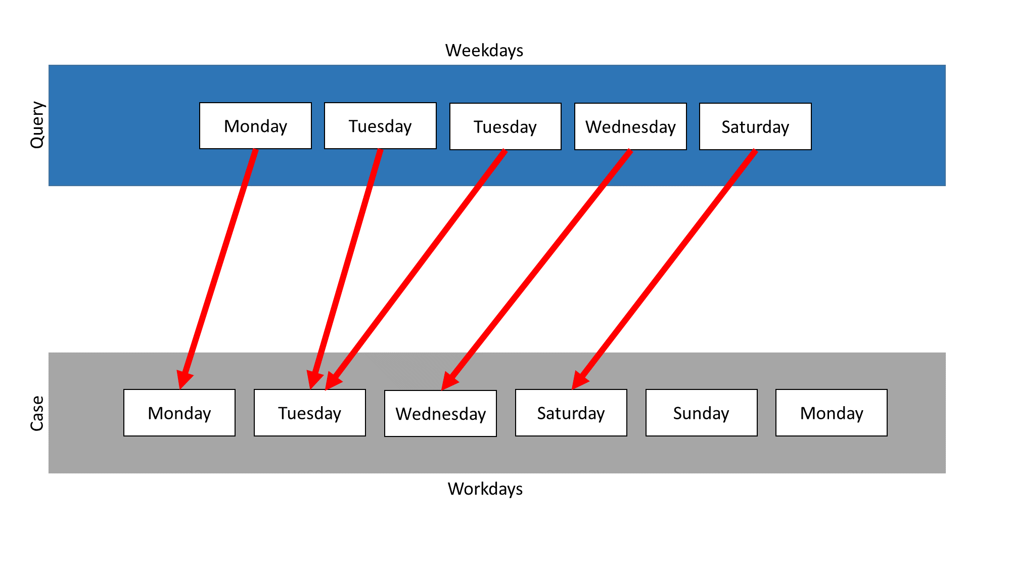
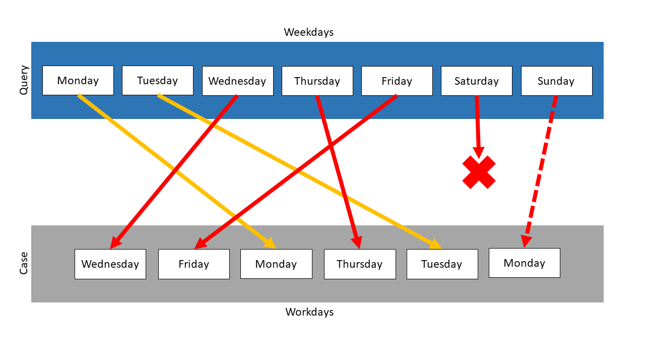
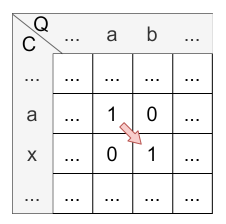
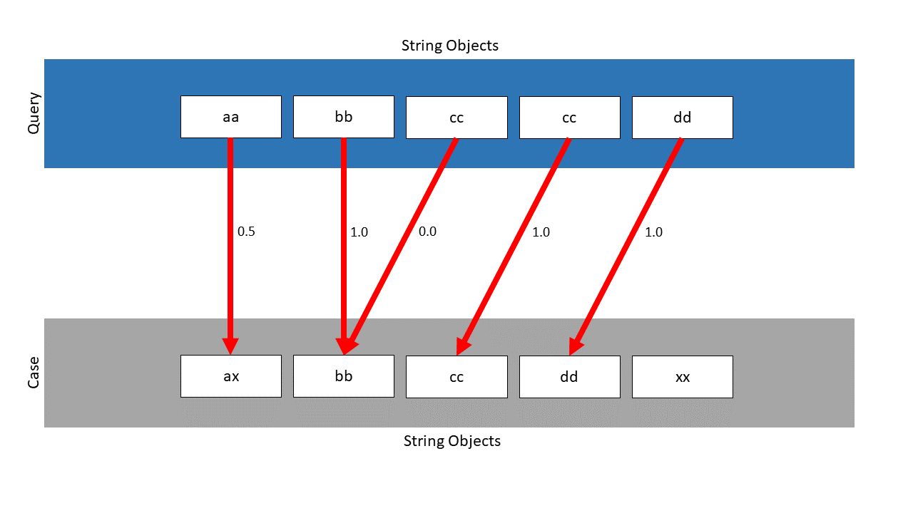
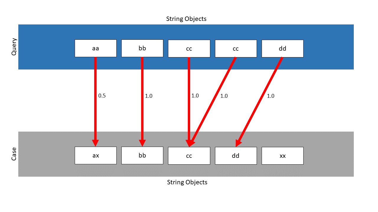
In the following example two collections exist, which are both objects of the class WeekdayList: The collection Weekdays contains all days from Monday until Sunday. The collection Workdays contains all workdays, Monday until Friday. The first example applies for both types of collection, namely lists or sets, as the order of the elements is not relevant.
In this example, the Isolated Mapping measure is used on those two collections. Weekdays is the query and Workdays the case. The following mapping results:
The measure searches for the most similar element in the case for each element in the query. The elements Monday, Tuesday, Wednesday, Thursday and Friday appear in query and case, so they are mapped on themselves. Thus, the similarity for each of these mappings is 1.0.
The elements Saturday and Sunday only occur in the query. They both need a mapping partner, so the measure searches for the most similar element in the case. In this example, Sunday is mapped on Monday and Saturday on Friday. The mappings of these elements depend on the similarity measures, which are used for the comparison of the elements. So this mapping is just one possibility. It was chosen, because Monday and Sunday have the highest Levenshtein similarity. Saturday is also compared with every element in the case, but is equal similar to all elements except Wednesday. In this case Friday was chosen randomly.
The overall similarity of both collections is computed by summing up single similarities using the Levenshtein measure in this example. The similarity value of Monday, Tuesday, Wednesday, Thursday and Friday is 1.0. The similarity between Sunday and Monday would be \(\frac{2}{3}\) and between Saturday and Friday would be \(\frac{1}{2}\) . So the total similarity would be calculated like this:
\(\frac{1.0 + 1.0 + 1.0 + 1.0 + 1.0 + \frac{2}{3} + \frac{1}{2}}{7} = 0.881\)If the String equals measure would be used, Saturday and Sunday would have random partners. These mappings would have the similarity 0.0, so the total similarity would be \(\frac{5}{7}\) .
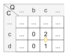
As seen in this example, the Isolated Mapping measure can map several query items on one case item. In an extreme case, it can happen, that all query items are mapped on just one element of the case, as can be seen in the next example.
Here, the collection Weekdays is used again, but this time as case. The query is a list, which contains the Monday item 5 times. It has to be a list, because a set, as the other existing type of collection, does not allow one element to appear several times.
Following mapping results:
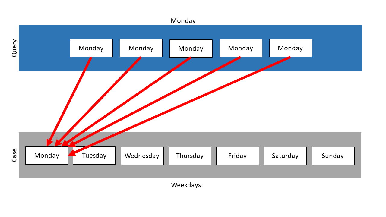
The item Monday is mapped on the Monday element in the case for 5 times. The resulting similarity is 1.0.
Mapping #
The measure performs the best possible mapping of two collections using the A* algorithm. It performs a best possible mapping of the query items to the case items of the collection. Note that not all case items have to be utilized in the mapping, but all query items are tried to map. Each query element can only be mapped on a case element, which has no mapping partner, yet. If more query items than case items exist, some query items will get a similarity 0 (which will influence the overall similarity). If more case items than query items exist, then this will not interfere with the similarity-value (rather gives more possible match-scenarios).
A restriction for the A* search can be set by using the parameter maxQueueSize. It is a restriction for the size of the internal queue of the A* algorithm. It can be used, to reduce the runtime, but can then also cause the best possible mapping not to be found. Its default value is 1000. It requires values larger than 0. If a negative value is set, the pruning of the queue is disabled. In this case, the optimal mapping will be found, but the runtime won’t be limited.
The following parameters can be set for this similarity measure.
| Parameter | Type/Range | Default Value | Description |
|---|---|---|---|
| similarityToUse | Similarity Measure (String) | null | The parameter is used to define, which similarity has to be taken for the similarity computation between the elements of the collections. For all elements, this one local measure will be used and afterwards the global similarity is aggregated. The similarity measure, which is referred, must exist in the runtime domain, too. Otherwise, an exception will be thrown. If no similarityToUse is defined, a usable data class similarity will be searched. If this one can’t be found, too, an invalid similarity will be returned. |
| maxQueueSize | Size (int) | 1000 | This parameter is a restriction for the size of the internal queue of the A* algorithm. It can be used, to reduce the runtime, but can then also cause the best possible mapping not to be found. It requires values larger than 0. If a negative value is set, the pruning of the queue is disabled. In this case, the optimal mapping will be found, but the runtime won’t be limited. |
The definition of a Mapping measure can look like:
<CollectionMapping name="SMCollectionMapping" class="WeekdayList" similarityToUse="SMStringEquals" maxQueueSize="1100"/>
To create this measure during runtime, the following code would be used:
    SMCollectionMapping smCollectionMapping = (SMCollectionMapping) simVal.getSimilarityModel().createSimilarityMeasure(
      SMCollectionMapping.NAME,
      ModelFactory.getDefaultModel().getClass("WeekdayList")
    );
    smCollectionMapping.setSimilarityToUse("SMStringEquals");
    smCollectionMapping.setMaxQueueSize(1100);
    simVal.getSimilarityModel().addSimilarityMeasure(smCollectionMapping, "SMCollectionMapping");
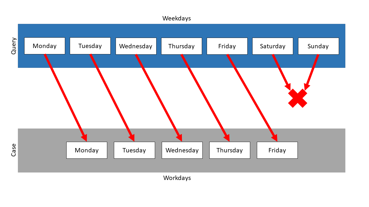
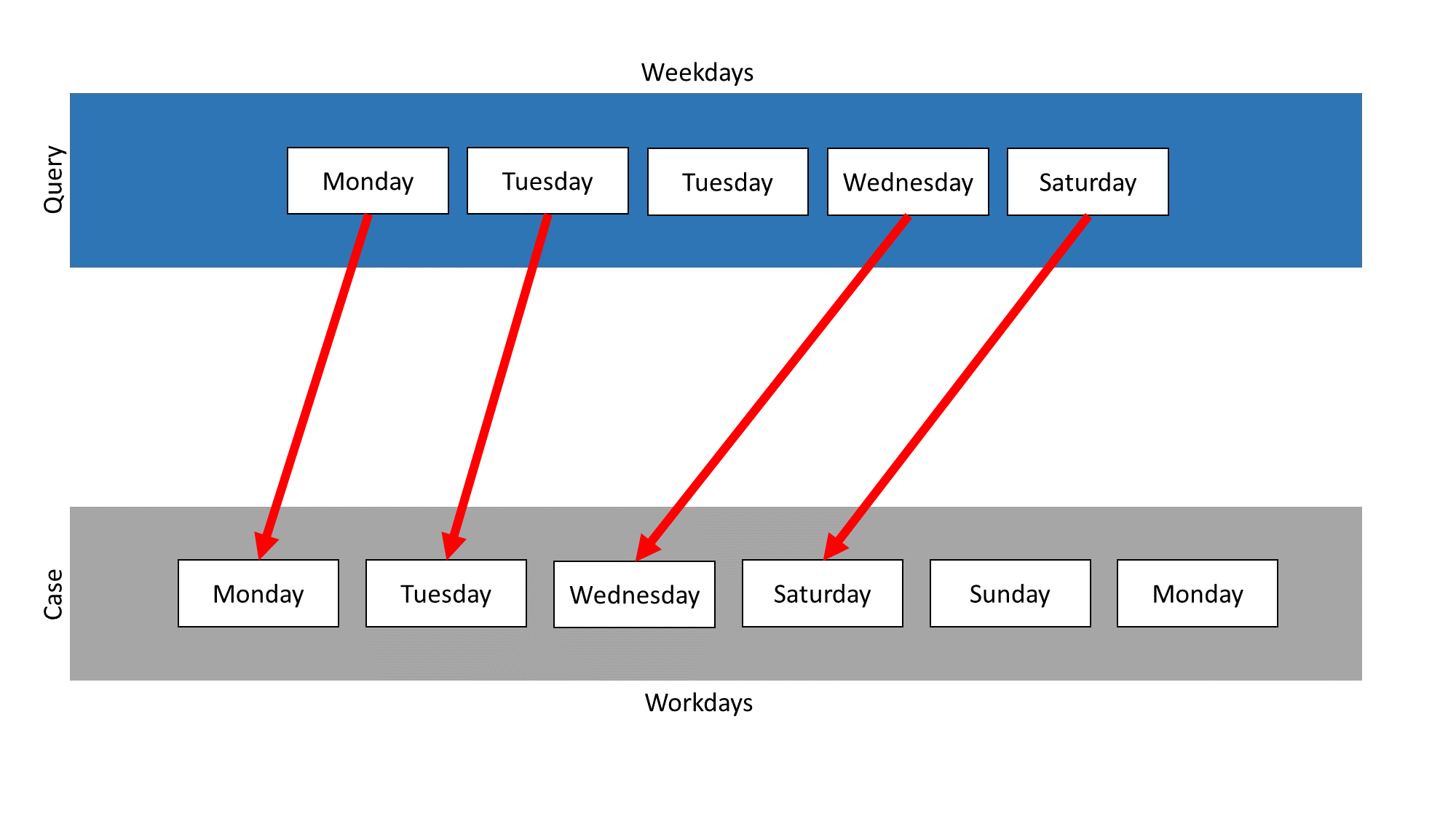
In this example two collections exist: The collection Weekdays contains all days from Monday until Sunday. The collection Workdays contains all workdays, Monday until Friday. It neither matters, if the collections are lists or sets, nor is the order important.
In this example, the Mapping measure is used on those two collections. Weekdays is the query and Workdays the case. Following mapping results:
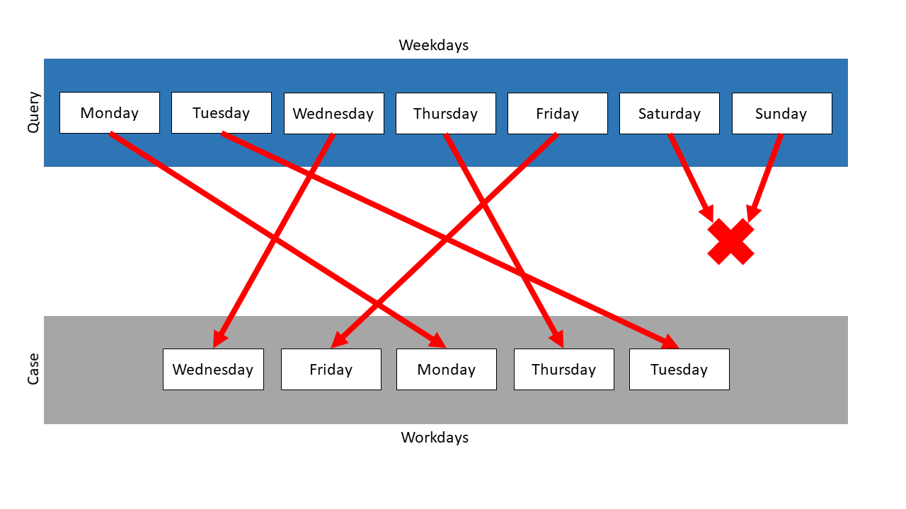
The measure searches the mapping partner with the highest similarity for every element of the query. Then the similarities are compared and the mapping with the highest similarity is chosen, the other mappings are not considered anymore. The search for mapping partners restarts, but neither the mapped query item nor the mapped case element are used anymore. So, in this example, Saturday and Sunday have no mapping partner, because for each case element exists a query partner with a higher similarity.
Because the query items were mapped on their representations in the case, the similarity of each of these mappings is 1.0. Saturday and Sunday could not be mapped, so they are treated like their mapping has the similarity 0.0. So the total similarity is \(\frac{5}{7}\) . In this example, the similarity is independent of the measure, which was used for the comparison of the items.
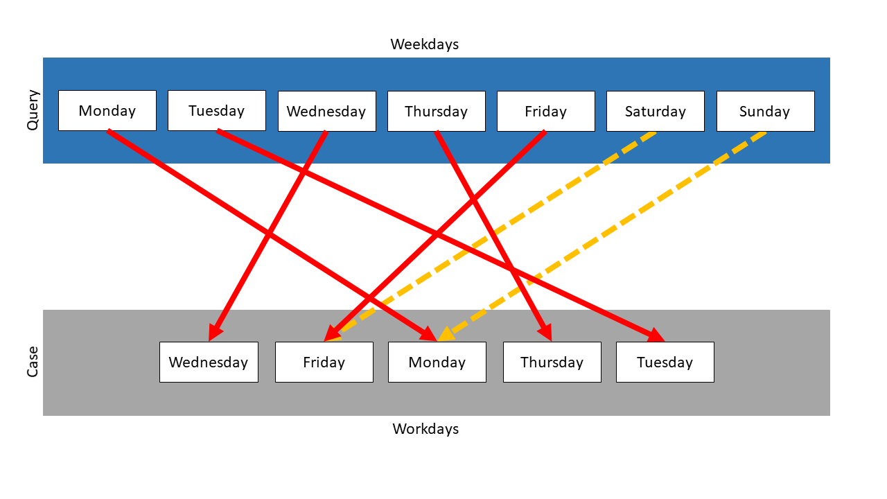
In the following is a second example. The element Monday is added to the collection Workdays. Because there is already one Monday in it, this collection must be a list. Weekdays again represents the query and Workdays the case.
The following mapping results:
Unlike the first example, there is now one available mapping partner for Saturday and Sunday. The Monday item of the query is mapped on one of the Monday items in the case, which is chosen randomly. The Monday item without a current mapping partner is compared to each query item. This repeats until the similarity value for the mapping of this item with Saturday or Sunday becomes the highest similarity. The mapping of this Monday element depends on the measure, which is used for the item comparison.
In the example above, the Levenshtein measure was used, so Monday was most similar to Sunday. The similarity between these elements is \(\frac{2}{3}\) , so the total similarity is computed like: \(\frac{1.0 + 1.0 + 1.0 + 1.0 + 1.0 + \frac{2}{3} + 0.0}{7} = 0.81\)
If the String equals measure would be used, Saturday would be the mapping partner of Monday, because it’s the first computation by this order. So the total similarity for this case is \(\frac{5}{7}\) .
ListWeighted #
The use of the similarity measures is that low similarity values can be penalized more and therefore a higher differentiation can be achieved. The mentioned “similarity values” are localSimilarities from the similarity calculation of the super class which are in turn weighted with ListWeights.
Currently, there are three different ListWeighted similarity measures: ListMappingWeighted, ListSWAWeighted and ListDTWWeighted. The following sections describe the general use of ListWeighted similarity measures. The specific use of the three measures is described in the respective sections.
ListWeight #
The ListWeights specify the interval in which they take effect and the value with which the similarities are to be evaluated.
The following parameters can be set:
| Parameter | Type/Range | Default Value | Description |
|---|---|---|---|
| listWeight | double | required | This parameter specifies the weighting with which the interval changes the similarities within it. |
| lowerBound | double [0,1] | required | This parameter indicates where the lower bound of the interval lies. |
| upperBound | double [0,1] | required | This parameter indicates where the upper bound of the interval lies. |
| lowerBoundInclusive | boolean | true | This parameter indicates whether the lowerBound is considered inclusive or exclusive. |
| upperBoundInclusive | boolean | true | This parameter indicates whether the upperBound is considered inclusive or exclusive. |
listWeight, lowerBound and upperBound are required parameters, without them there is no object instantiation possible. There do not exist default values.
The representation of a ListWeight object in XML can look like:
<!-- This instatiation does not work in XML, because <Weight.../> is only allowed in between a ListWeighted similarity measure!  -->
<Weight listWeight="2.0" lowerBound="0.8" upperBound="0.9" lowerBoundInclusive="false" upperBoundInclusive="true"/>
The creation at runtime can look like this:
ListWeight listWeight = new ListWeightImpl(2, 0.8, 0.9, false, false);
Implementation #
The only new parameter that the ListWeighted similarity measures have compared to the inherited similarity measures is the parameter listWeights.
| Parameter | Type/Range | Default Value | Description |
|---|---|---|---|
| listWeights | List of ListWeights | null | This parameter stores the weights of the similarity measure, there are 2 ways to set the weights: - add the weights one after the other (using addWeight(ListWeight listWeight))- set a list of weights directly ( using setWeights(LinkedList<ListWeight> listWeights)) |
There are also some other methods to work with in ListWeighted similarity measures:
| Method | Description |
|---|---|
deleteWeight(int index) | This method deletes a ListWeight at a specific index. Note that the index of a particular ListWeight may have shifted after the similarity calculation, this is due to filling in missing weights and sorting the already introduced weights. For further information, have a look at shifting and filling up ListWeights. |
removeAllWeights() | This method is used to reuse the same similarity measure by removing all previous weights and allowing new ones to be added. |
Calculation #
For the weighted similarity calculation to work, first all weights are sorted by ascending interval value, then missing weights are filled up and finally normalized. It does not matter in which order the ListWeights are added. It is also possible to omit intervals, these are then added as interval using the given default weight. The normalization means that the smallest value (!= 0) is increased/decreased to the value 1. The other weights are then also changed proportionally.
An abstracted use case of this behavior can look like this:
weight=0.8, range: [0.8, 1.0]
weight=0.2, range: (0.7, 0.8)
The weights are sorted and missing weights are filled up at the right positions:
weight=0.0, range: [0.0, 0.7]
weight=0.2, range: (0.7, 0.8)
weight=0.8, range: [0.8, 1.0]
Finally, the weights of the intervals are normalized as described above:
weight=0.0, range: [0.0, 0.7]
weight=1.0, range: (0.7, 0.8)
weight=4.0, range: [0.8, 1.0]
Lists like the following leading to Exceptions:
// overlap of intervals
weight=0.0, range: [0.0, 0.7]
weight=3.0, range: [0.6, 0.8]
// non existing interval
weight=0.0, range: (0.1, 0.1)
The similarity calculation is based on the local similarities generated from the superclass. For example, the
ListSWAWeighted calls the ListSWA and then weights these local similarities to a final similarity.
The overall global similarity is always computed based on the following formula:
Therefore, the mappings made by the respective algorithm are taken and the local similarities calculated between these are used for the similarity calculation.
A detailed examination of the similarity calculation reveals that, initially, a weighting calculation is conducted for each local similarity. For instance, when considering values from the given example, if a similarity score is 0.9, it falls within the interval [0.8, 1.0] and is multiplied by the factor \(\frac{currentWeight}{maxWeight} = \frac{w_{sim_{local} (q,c)}}{w_{max}}\) , here \(4/4\) . This implies that similarities within the interval with the highest weighting are incorporated into the final similarity at a 100% contribution. Alternatively, if a similarity has a value of \(0.75\) , it falls within the interval (0.7, 0.8) with a weight of \(1.0\) . In this case, the local similarity is multiplied by the value \(1/4\) , indicating that similarities within the interval (0.7, 0.8) only contribute to the final similarity with 25% influence. If these are the only two similarities present, the sum of the weighted local similarities is calculated and divided by the total influence factor, which in this scenario is 125% (i.e., 1.25). In summary, the calculation involves \( \frac{1.0 * \frac{4}{4} + 0.75 * \frac{1}{4}}{1.25} \) .
List Mapping #
The List Mapping measure compares two lists and also considers the order of elements. Other collection types are not supported. The similarity between two lists can be computed with two different meanings:
- Exact: This means, that the two lists must have the same length to be compared. Each element is compared with the element at the same position in the other list. The similarities for each comparison are summed and divided through the length of the list.
- Inexact: This means, that one of the two lists can be a sublist of the other. The similarities for possible sublists are computed like in the exact comparison. In the end, the best similarity is reported. In both cases the measure follows the exact order of the list.
The following parameters can be set for this similarity measure.
| Parameter | Type/Range | Default Value | Description |
|---|---|---|---|
| similarityToUse | Similarity Measure (String) | null | The parameter is used to define, which similarity has to be taken for the similarity computation between the elements of the collections. For all elements, this one local measure will be used and afterwards the global similarity is aggregated. The similarity measure, which is referred, must exist in the runtime domain, too. Otherwise, an exception will be thrown. If no similarityToUse is defined, a usable data class similarity will be searched. If this one can’t be found, too, an invalid similarity will be returned. |
| contains | Flag (String) | inexact | This parameter defines the meaning of the comparison of two lists. If it’s set to exact, the two lists must have the same length to be compared. Each element is compared with the element at the same position in the other list. The similarities for each comparison are summed and divided through the length of the list. If the parameter is set to inexact, one of the two lists can be a sublist of the other. The similarities for possible sublists are computed like in the exact comparison. In the end, the best similarity is reported. In both cases the measure follows the exact order of the list. |
| returnLocalSimilarities | Flag (boolean) | true | This parameter modifies the returned similarity object of query and case, if this parameter is set to true, the local similarities are added to the similarity object of query and case. |
The definition of a List Mapping measure can look like:
<ListMapping name="SMListMapping" class="WeekdayList" contains="exact" similarityToUse="SMStringEquals" default="false" returnLocalSimilarities="false"/>
To create this measure during runtime, the following code would be used:
    SMListMapping smListMapping = (SMListMapping) simVal.getSimilarityModel().createSimilarityMeasure(
      SMListMapping.NAME,
      ModelFactory.getDefaultModel().getClass("WeekdayList")
    );
    smListMapping.setContainsExact();
    smListMapping.setReturnLocalSimilarities(false);
    smListMapping.setSimilarityToUse("StringEqualsCaseSensitive");
    simVal.getSimilarityModel().addSimilarityMeasure(smListMapping, "SMListMapping");
Here, the collection class WeekdayList and the StringEquals similarity have to be defined somewhere else.
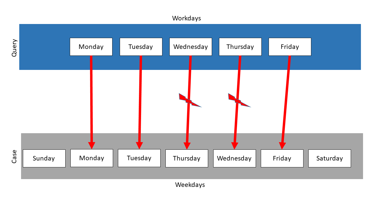
In this example two lists exist: The list Weekdays contains all days from Monday until Sunday. The list Workdays contains all workdays, Monday until Friday. This measure works only on lists, so sets are not mentioned here.
In the following, List Mapping is used on the two lists. The following mapping results:
The sizes of the lists are different, so some items cannot be mapped. When using the exact mapping strategy, the similarity would be 0.0.
The inexact mapping strategy ignores the sizes of the lists. So it is checked, whether one list is a sublist of the other. In this example, three possible sublists are found. For each of them, the total similarity is computed, and the one with the highest similarity is chosen. Here, Workdays is a sublist of Weekdays, so the similarity is 1.0 and this mapping is chosen.
In the following is a second example. Here, Workdays is the query and Weekdays the case. But the order of Weekdays is different, so Thursday and Wednesday swapped their positions.
When using the exact mapping strategy, the similarity would be 0.0 and no mapping would be tried. So the following mapping just results, when using the inexact mapping strategy:
The measure finds three sublists again and computes the similarities. It identifies the second to the sixth element as the mapping partners with the highest similarity. But this measure follows the exact order of the items. So the element Wednesday is mapped on Thursday, just as Thursday on Wednesday. So, when using the String equals measure, the similarity is \(\frac{3}{5} = 0.6\) .
ListMappingWeighted #
Before reading on, please first read the basic information about the ListWeighted similarity measures.
The similarity measure ListMappingWeighted uses the similarity measure ListMapping as a basis. Here, local similarities are created, which are then used in ListMappingWeighted to offset them with the matching ListWeights.
In XML this measure can be defined as follows:
    <ListMappingWeighted name="SMListMappingWeightedXML" class="CustomListClassXML" defaultWeight="1.0" similarityToUse="CustomStringLevenshteinXML" returnLocalSimilarities="false">
        <Weight listWeight="1.0" lowerBound="0.0" upperBound="0.1"/>
        <Weight listWeight="2.0" lowerBound="0.1" upperBound="0.6" lowerBoundInclusive="false" upperBoundInclusive="true"/>
        <Weight listWeight="4.0" lowerBound="0.6" upperBound="1.0" lowerBoundInclusive="false" upperBoundInclusive="true"/>
    </ListMappingWeighted>
At creation during runtime, the following code can be used:
    SMListMappingWeighted listMappingWeighted = (SMListMappingWeighted) simVal.getSimilarityModel().createSimilarityMeasure(
                SMListMappingWeighted.NAME, firstList.getDataClass()
    );
    listMappingWeighted.setSimilarityToUse("CustomStringLevenshtein");
    listMappingWeighted.setReturnLocalSimilarities(false);
    simVal.getSimilarityModel().addSimilarityMeasure(listMappingWeighted, "SMListMappingWeighted");

    listMappingWeighted.addWeight(new ListWeightImpl(1.0, 0.0, 0.1));
    listMappingWeighted.addWeight(new ListWeightImpl(2.0, 0.1, 0.6, false, true));
    listMappingWeighted.addWeight(new ListWeightImpl(4.0, 0.6, 1.0, false, true));
Example #
As local similarity measure the StringLevenshtein is used and the ListClass is utilized. Furthermore, the following intervals are given:
weight=1.0, range: [0.0, 0.1]
weight=2.0, range: (0.1, 0.6]
weight=4.0, range: (0.6, 1.0]
The ListMapping finds the following mapping, the local similarities are located next to the pawls:
Without the weighted approach, the similarity would be: \(\frac{2.5}{5} = 0.5\) . Considering the weights, the following similarity is calculated: \(\frac{0.5 \cdot \frac{2}{4} + 1.0 \cdot \frac{4}{4} + 1.0 \cdot \frac{4}{4} + 0.0 \cdot \frac{1}{4} +0.0 \cdot \frac{1}{4}}{\frac{2}{4} + \frac{4}{4} + \frac{4}{4} + \frac{1}{4} +\frac{1}{4}} = 0.75\) . As can be seen, the similarity has been increased from \(0.5\) to \(0.75\) .
List Correctness #
The List Correctness measure compares two lists by the order of their elements. Other collection types aren’t supported.
This similarity measure uses the Correctness metric to compare two lists. This metric is the ratio of concordant and discordant pairs regarding all pairs. Its value is usually in the range of \(-1\)
to \(1\)
. \(-1\)
means, that only discordant pairs are given and \(1\)
means that only concordant pairs are given. Values in the range of \([0,1]\)
are used directly as similarity values. For values in the range of \([-1.0)\)
, a parameter discordantParameter \(p_{d}\)
can be set. It defines the maximum possible similarity, if a correctness of \(-1\)
would be reached. The similarity values decrease linearly between this value till 0. The default value for this parameter is \(1.0\)
.
The meaning of concordant and discordant pairs is described here.
The similarity is computed by the following formula
\(sim_{correctness} = \begin{cases} \frac{|C|-|D|}{|C|+|D|}, &\text{if} \ |C| \geq |D|\\ \\ \bigl|\frac{|C|-|D|}{|C|+|D|}\bigl| \ * \ p_{d}, &\text{if} \ |C| < |D|\\ \end{cases}\)The following parameters can be set for this similarity measure.
| Parameter | Type/Range | Default Value | Description |
|---|---|---|---|
| discordantParameter | Weight (double) | 1.0 | This parameter defines the maximum possible similarity, if a correctness of \(-1\) would be reached. The similarity values decrease linearly between this value till 0. |
The definition of a List Correctness measure can look like:
<ListCorrectness name="SMListCorrectness" class="WeekdayList" discordantParameter="0.5" default="false"/>
To create this measure during runtime, the following code would be used:
    SMListCorrectness smListCorrectness = (SMListCorrectness) simVal.getSimilarityModel().createSimilarityMeasure(
      SMListCorrectness.NAME,
      ModelFactory.getDefaultModel().getClass("WeekdayList")
    );
    smListCorrectness.setDiscordantParameter(0.5);
    simVal.getSimilarityModel().addSimilarityMeasure(smListCorrectness, "SMListCorrectness");
In this example two lists exist: The first list contains all days from Monday until Wednesday in order of the week. The second list contains the days in the following order: Monday, Wednesday, Tuesday. Here, the order of the element Monday to the element Tuesday and of Monday to the element Wednesday matches. So, two concordant pairs can be found. Only the order of the element Tuesday to the element Wednesday doesn’t match. So, this pair is discordant. Because more concordant than discordant pairs does exits, the following similarity would be computed: \(\frac{2-1}{2+1}=\bigl\frac{1}{3}\) .
In another example, the first list containing the three days in order of the week exist, too. An additional list contains these elements in reverse order: Wednesday, Tuesday, Monday. Here, all elements occur in a different order. So, only discordant pairs could be computed. With no discordantParameter set, the following similarity would be computed: \(\bigl|\frac{0-3}{0+3}\bigl| * 1= \bigl|-1\bigl| \ * \ 1 = 1\)
. If the parameter was set to \(0.5\)
, the similarity would be computed as follows: \(\bigl|\frac{0-3}{0+3}\bigl| \ * \ 0.5= \bigl|-1\bigl| \ * \ 0.5 = 0.5\)
Smith Waterman Algorithm (SWA) #
Lists can be regarded as time series. Therefore, the Smith Waterman Algorithm (SWA) based on sequence matching has been adapted for comparing two list objects. This measure can be seen as an extension to the basic ListMapping. The SWA is based on the Needleman-Wunsch Algorithm and is able to find local alignments of two data sequences, the alignment is completed when the best matching sub-sequences are identified. These alignments are constructed by iteratively either aligning, inserting or deleting elements from one series with regard to the other. The approach therefore is somewhat similar to the Levenshtein distance approach. In the following, the individual characteristics of the SWA is outlined and the implementation and integration in ProCAKE is described.
In the following, the SWA is explained with its default parameters, later there are several modifications of the SWA described.
SWA calculates the alignment and thereupon the similarity score in the following way:
First, the scoring matrix \(H\) is initialized. The query \(Q\) which is a list of elements with length \(|Q|\) is indexed using \(i = 1,...,|Q|\) and case \(C\) which is also a list of elements with length \(|C|\) is indexed by \(j = 1,...,|C|\) . With this convention, \(q_i\) depicts the i-th character from \(Q\) . \(q_0\) and \(c_0\) are identified with the gap character \(\text{'}-\text{'}\) and the first row and column of the matrix are set to zero: \(H_{0,j}=H_{i,0}=0\) . Entry \(H_{i,j}\) is interpreted as the subsequence similarity of \(q'_i = q_1 q_2 .. q_i\) and \(c'_j = c_1 c_2 .. c_j\) for \(i,j > 0\) . When either \(i=0\) or \(j=0\) , then \(q_0=\text{'}-\text{'}\) or \(c_0=\text{'}-\text{'}\) and hence, similarity of a list with the empty list is set to 0.
The scoring matrix is filled in according to the following formula:
\( H_{i,j} = \text{max} \begin{cases} \quad 0, \\ \quad H_{i-1,j-1} + sim(q_i,c_j), &\text{match/mismatch}\\ \quad H_{i-1,j} - 1, &\text{deletion}\\ \quad H_{i,j-1} - 1 &\text{insertion} \end{cases} \)
The function \(sim\) represents a similarity measure that can be applied to compare the elements of the collection and is specified as parameter of the SWA.
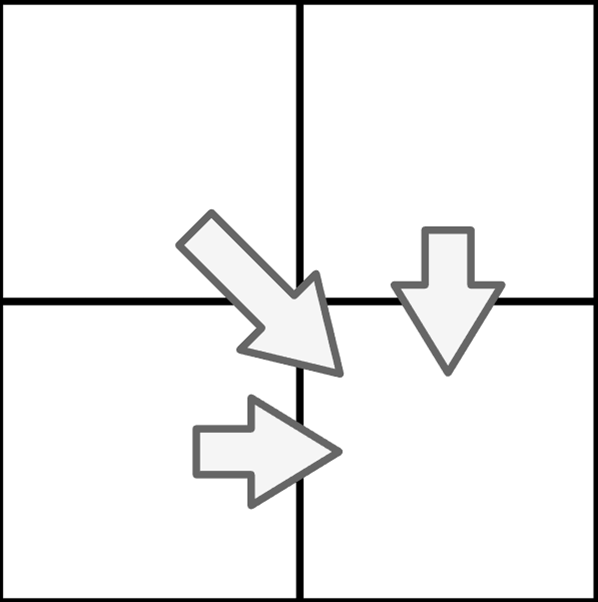
A match corresponds to a diagonal, an insertion to a vertical and a deletion to a horizontal step in the matrix. The values’ origins must be stored during calculation if one wants to visualize the optimal alignment later.
- In order to obtain the alignment, one has to find the maximum value in the last column in the matrix and trace back a path to a cell where the query is indexed with 0 (the gap character). This is done by successively stepping either vertically to the top, horizontally to the left or diagonally to the top left adjacent cell according to the inverted direction of the initial score calculation. The alignment path is always unique.
Introductory example #
In this example the parameters of the SWA are not modified in any way, all the default values are used.
For the function \(sim\)
, a simple StringEquals similarity measure, therefore \(sim\)
is defined as follows:
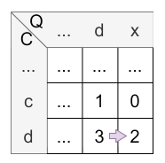
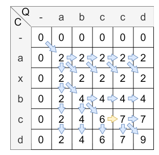
Let Q = [a,b,c,d,x] and C = [a,x,b,c,d] be lists of characters.
Initialization
According to the above steps, first the scoring matrix has to be initialized:
Calculation
The next step is to fill the matrix with the values. The following figure shows the matrix after the calculation:
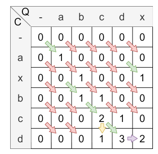
The yellow arrow clarifies the insertion and the purple arrow clarifies the deletion. The green arrows are showing the matches, the red ones the mismatches.
A cell can be computed in four different ways:
- match (diagonal jump, calculation: \(H_{i-1,j-1} + 1\) )
- mismatch (diagonal jump, calculation: \(H_{i-1,j-1}\) )
- deletion (horizontal, calculation: \(H_{i-1,j} - 1\) )
- insertion (vertical, calculation: \(H_{i,j-1} - 1\) )
There is just one condition: The lower right field must be at maximum. If all calculation ways resulting in the same value, diagonal comes before horizontal and horizontal comes before vertical, when determining the origin of the score.
To reach this, the maximum from the four possible calculation ways is chosen.
Let’s have a look at the calculation of cell \(H_{1,1}\) :
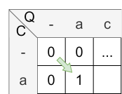
- match: \(H_{0,0} + sim(a,a) = 0 + 1 = 1\)
- mismatch: There is no mismatch.
- deletion: \(H_{0,1} - 1 = 0 - 1 = 0\) (note that \(H_{i,j} \) is never less than 0 caused by its definition)
- insertion: \(H_{1,0} - 1 = 0 - 1 = 0\) (note that \(H_{i,j} \) is never less than 0 caused by its definition)
The maximum is 1, so the match (diagonal) is applied and the value of \(H_{1,1}\) is 1. The origin of \(H_{1,1}\) is \(H_{0,0}\) caused by the diagonal jump.
Let’s have a look at the calculation of cell \(H_{2,2}\) :
- match: There is no match.
- mismatch: \(H_{1,1} = 1 = 1\)
- deletion: \(H_{1,2} - 1 = 0 - 1 = 0\) (note that \(H_{i,j} \) is never less than 0 caused by its definition)
- insertion: \(H_{2,1} - 1 = 0 - 1 = 0\) (note that \(H_{i,j} \) is never less than 0 caused by its definition)
The maximum is 1, so the mismatch (diagonal) is applied and the value of \(H_{2,2}\) is 1. The origin of \(H_{2,2}\) is \(H_{1,1}\) caused by the diagonal jump.
Let’s have a look at the calculation of cell \(H_{3,5}\) :
- match: There is no match.
- mismatch: \(H_{2,4} = 0 = 0\)
- deletion: \(H_{3,4} - 1 = 0 - 1 = 0\) (note that \(H_{i,j} \) is never less than 0 caused by its definition)
- insertion: \(H_{2,5} - 1 = 2 - 1 = 1\)
The maximum is 1, so the insertion (vertical) is applied and the value of \(H_{3,5}\) is 1. The origin of \(H_{3,5}\) is \(H_{3,4}\) caused by the vertical jump.
Let’s have a look at the calculation of cell \(H_{5,5}\) :
- match: There is no match.
- mismatch: \(H_{4,4} = 1 = 1\)
- deletion: \(H_{4,5} - 1 = 3 - 1 = 2\)
- insertion: \(H_{5,4} - 1 = 0 - 1 = 1\) (note that \(H_{i,j} \) is never less than 0 caused by its definition)
The maximum is 1, so the insertion (horizontal) is applied and the value of \(H_{5,5}\) is 1. The origin of \(H_{5,5}\) is \(H_{4,5}\) caused by the horizontal jump.
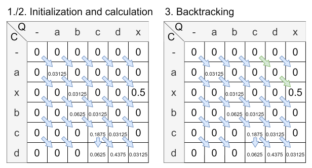
Backtracking
In the last step, the cell with the highest value in the last column is the starting point of the backtracking. From there, the path is traced back to the cell where the query is indexed with 0 (the gap character). \(H_{0,x}\) for \(x \in |C|\) are all possible ending points of the alignment path. In this example, the ending point of the alignment path is \(H_{0,1}\) . The alignment path is shown in the following figure:
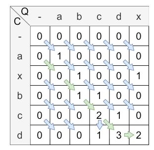
The alignment path is always unique. This path is used to calculate the similarity score. The similarity score is calculated by dividing the value of the last element from the alignment path (2) by the length of the alignment path (5). Therefore, the overall similarity score is \(\frac{2}{5} = 0.4\) .
Note that this example is based on the default values. The default values can be changed, which means that some procedures described here are no longer valid. However, this is described in more detail in the next chapter.
Implementation of the calculation #
The implementation of the SWA is more complex and allows for a configuration through parameters.
The matrix is constructed using the following formula:
\(H_{i,j} = max \begin{cases} \quad H_{i-1,j-1} + \ wTemp_i * sim_{loc}(q_i,c_j)& \text{if } x=\text{'diagonal'},\\ \quad H_{i-1,j} + \ wTemp_i * deletionPenalty(q_i)& \text{if } x=\text{'horizontal'},\\ \quad H_{i,j-1} + \ wTemp_i * insertionPenalty(c_j)& \text{if } x=\text{'vertical'},\\ \quad 0& \text{otherwise} \end{cases}\)\(q_i\)
represents the i-th query item and \(c_j\)
the j-th case item. \(sim_{loc}\)
is the local similarity measure used. The parameters constInsertionPenalty and constDeletionPenalty can also be set by the user, both are -1 by default.
If the parameter halvingDistance is not set, \(wTemp_i\)
is equal to 1.0 and has no effect on the calculation of the matrix. Therefore, \(wTemp\)
was not introduced in the introductory example. If the parameter halvingDistance is set, read more about the calculation of wTemp here.
Given the constructed scoring matrix, the final non-normalized similarity is calculated as follows:
\(sim_{raw}(q,c) = \max_{0 < j \leq m} H_{n,j}\)With \(m\)
as the length of the case instance, this ensures that the alignment always ends with the last task of the query. Note that this behavior can be changed by setting the parameter endWithQuery.
For the SWA, the maximum similarity score is achieved when all elements are mapped. Thus, for all elements of the query, the weighting factors are summarized, assuming a similarity of 1. This value is used for normalization:
\(sim^{SWA}_{normed}(q, c) = \frac{sim_{raw}(q,c)}{\displaystyle\sum^{i<n}_{i=0} wTemp_i} \\\)Measure instantiation and configuration #
For this SWA-based measure, the following parameters can be set.
| Parameter | Type/Range | Default Value | Description |
|---|---|---|---|
| endWithQuery | Flag (boolean) | true | This parameter specifies whether the last item of the query must be in the alignment path. |
| halvingDist | Percentage (Double, [0,1]) | 0.0 | This parameter specifies the distance to the end where the events’ importance shall be one half. |
| constInsertionPenalty | Functional interface | t -> -1.0 | This parameter is used to define a functional interface that gets the specific item being inserted as input. The output must be a negative numeric value. Note that, in xml, only constant values can be specified. |
| constDeletionPenalty | Functional interface | t -> -1.0 | This parameter is used to define a functional interface that gets the specific item being inserted as input. The output must be a negative numeric value. Note that, in xml, only constant values can be specified. |
| localSimName | Similarity Measure (String) | null | The parameter is used to define, which similarity has to be taken for the similarity computation between the elements of the collections. For all elements, this one local measure will be used and afterwards the global similarity is aggregated. The similarity measure, which is referred, must exist in the runtime domain, too. Otherwise, an exception will be thrown. If no localSimName is defined, a usable data class similarity will be searched. If this neither can be found, an invalid similarity will be returned. |
| ignoreDifferentBeginnings | Enumeration (String) | IGNORE_DIFFERENT_BEGINNINGS_CASE | This parameter changes the similarity measure so that different beginnings are taken into account in the similarity calculation. It is possible to consider different beginnings in the case (IGNORE_DIFFERENT_BEGINNINGS_CASE), in query and case (IGNORE_DIFFERENT_BEGINNINGS_CASE_AND_QUERY) or to consider no different beginnings at all (NONE). |
| localSimilarities | Flag (boolean) | false | This parameter modifies the returned similarity object of query and case, if this parameter is set to true, the local similarities are added to the similarity object of query and case. |
The SWA-based measure can be instantiated during runtime as follows:
    SMListSWA smListSWA = (SMListSWA) simVal.getSimilarityModel().createSimilarityMeasure(
      SMListSWA.NAME,
      ModelFactory.getDefaultModel().getClass("WeekdayList")
    );
    simVal.getSimilarityModel().addSimilarityMeasure(smListSWA, "SMListSWA");
The similarity measure can be configured using the following parameters:
endWithQuery #
By default, the final alignment must include the last item of the query, however, this behavior can be disabled:
smListSWA.setForceAlignmentEndsWithQuery(false);
false and let A = “abcd” and B = “ab”, then the scoring matrix including alignment path looks as follows: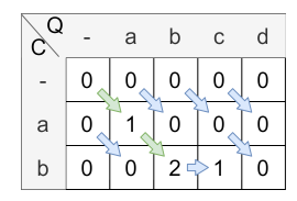
The alignment starts at the maximal value in the matrix and is traced back to its origin.
halvingDist #
If the parameter halvingDistance is not set, \(wTemp_i\)
is equal to 1.0.
If the parameter halvingDistance is set, it allows for temporal weighting of the similarities with the following formula:
\( wTemp_i = \frac{1}{2^\frac{n-i}{round(n \cdot h)}}
\)
.
- \(n\) is the length of the query.
- \(round()\) rounds a decimal number to the nearest whole number.
- \(h\) is the halving distance and specifies the distance to the end where the events’ importance shall be one half.
Therefore, with this formula, the weight of an event at the end of the sequence will be one, the weight of an event at \(end - h\) will be one half, and the weight of an event prior to \(end - h\) will be between 0 and one half. By using this formula, differences in the series, that are closer to the end of the sequences, will be weighted higher than dissimilarities further in the past. The halving distance can be specified as a percentage value (denoted as a value from \([0,1]\) ) of the length of the query. The distance is measured starting from the end of the query.
To illustrate this further, the factor is used on the introductory example. To set the halving distance to 0.2, the following code is used:
smListSWA.setHalvingDistancePercentage(0.2);
The following figure shows the calculated matrix with the halving distance set to 0.2:
The final similarity is calculated by the already given formula: \( sim^{SWA}_{normed}(q, c) = \frac{sim_{raw}(q,c)}{\displaystyle\sum^{i<n}_{i=0} wTemp_i} = \frac{sim_{raw}(q,c)}{\displaystyle\sum_{i = 0}^{i < n}2^{\frac{n - i}{round(n \cdot h)}}} = \frac{0.5}{0.96875} \approx 0.516 \)
Comparing the introductory example with the similarity calculated using halvingDistance, one observes a change in the alignment path and an increased similarity with halvingDistance. This is attributed to the fact that the non-matching sequences at the beginning carry less weight, while the matching sequences further back in the query are given more emphasis.
constInsertionPenalty / constDeletionPenalty #
Insertion and deletion penalty schemes can be specified using a functional interface that gets the specific item being inserted or deleted as input. The output must be a negative numeric value.
    smListSWA.setInsertionScheme(t -> -0.5);
    smListSWA.setDeletionScheme(t -> -0.5);
localSimName #
When the local similarity to use is specified, this overwrites the configuration of the similarity model.
smListSWA.setLocalSimilarityToUse("SMStringEquals");
ignoreDifferentBeginnings #
It is possible to consider different beginnings of the similarity calculation. Possible values are: NONE, IGNORE_DIFFERENT_BEGINNINGS_CASE and IGNORE_DIFFERENT_BEGINNINGS_CASE_AND_QUERY. By default, the parameter is set to IGNORE_DIFFERENT_BEGINNINGS_CASE.
smListSWA.setIgnoreDifferentBeginnings(DIFFERENT_BEGINNINGS_STRATEGIES.IGNORE_DIFFERENT_BEGINNINGS_CASE);
In the introductory example, it is shown how the default value behaves, in the following the other options are described:
IGNORE_DIFFERENT_BEGINNINGS_CASE_AND_QUERY: Set with this parameter, the matrix of the introductory example would have been calculated in the following way: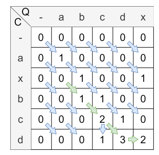
IGNORE_DIFFERENT_BEGINNINGS_CASE_AND_QUERY means, that if the first 0 is reached in the backtracking, the alignment path is finished and so the different beginnings are ignored.
The resulting similarity is \(\frac{2}{4} = 0.5\) .
NONE: If the parameter is set to NONE, the path is traced back until first row or column is reached. If the introductory example would be calculated with this parameter, there would be no difference, because the alignment path is already traced back to the first column.
localSimilarities #
It is possible to calculate the local similarities of query and case, these similarities are added to the similarity object of the query and case calculation.
smListSWA.setReturnLocalSimilarities(true);
Instantiation via XML is also possible, however, insertion and deletion penalty schemes can only be set to a constant value. Possible values for ignoreDifferentBeginnings are: none, ignore_different_beginnings_case and ignore_different_beginnings_case_and_query.
    <ListSWA name="SMListSWA"
        class="WeekdayList"
        halvingDist="0.2"
        localSimName="SMStringEquals"
        constInsertionPenalty="-0.5"
        constDeletionPenalty="-0.5"
        endWithQuery="false"
        ignoreDifferentBeginnings="none"
        returnLocalSimilarities="true"/>
ListSWAWeighted #
Before reading on, please first read the basic information about the ListWeighted similarity measures.
The similarity measure ListSWAWeighted uses the similarity measure ListSWA as a basis. Here, local similarities are created, which are then used in ListSWAWeighted to offset them with the matching ListWeights.
In XML this measure can be defined as follows:
    <ListSWAWeighted name="SMListSWAWeightedXML" class="CustomListClassXML" defaultWeight="0.0" localSimName="CustomStringLevenshteinXML">
        <Weight listWeight="1.0" lowerBound="0.0" upperBound="0.1"/>
        <Weight listWeight="2.0" lowerBound="0.1" upperBound="0.6" lowerBoundInclusive="false" upperBoundInclusive="true"/>
        <Weight listWeight="4.0" lowerBound="0.6" upperBound="1.0" lowerBoundInclusive="false" upperBoundInclusive="true"/>
    </ListSWAWeighted>
At creation during runtime, the following code can be used:
    SMListSWAWeighted listSWAWeighted = (SMListSWAWeighted) simVal.getSimilarityModel().createSimilarityMeasure(
                SMListSWAWeighted.NAME, firstList.getDataClass()
    );
    listSWAWeighted.setLocalSimilarityToUse("CustomStringLevenshtein");
    simVal.getSimilarityModel().addSimilarityMeasure(listSWAWeighted, "SMListSWAWeighted");

    listSWAWeighted.addWeight(new ListWeightImpl(1.0, 0.0, 0.1));
    listSWAWeighted.addWeight(new ListWeightImpl(2.0, 0.1, 0.6, false, true));
    listSWAWeighted.addWeight(new ListWeightImpl(4.0, 0.6, 1.0, false, true));
Example: #
As local similarity measure the StringLevenshtein is used and the ListClass is utilized. Furthermore, the following intervals are given:
weight=1.0, range: [0.0, 0.1]
weight=2.0, range: (0.1, 0.6]
weight=4.0, range: (0.6, 1.0]
The SWA finds the following mapping, the local similarities are located next to the pawls:
Without the weighted approach, the similarity would be: \(\frac{3.5}{5} = 0.7\) . Considering the weights, the following similarity is calculated: \(\frac{0.5 \cdot \frac{2}{4} + 1.0 \cdot \frac{4}{4} + 0.0 \cdot \frac{1}{4} + 1.0 \cdot \frac{4}{4} +1.0 \cdot \frac{4}{4}}{\frac{2}{4} + \frac{4}{4} + \frac{1}{4} + \frac{4}{4} +\frac{4}{4}} = 0.8\overline{6}\) . By choosing the right weights, the smaller similarities are only of minor importance and therefore an increased final similarity can be achieved. As can be seen, the similarity has been increased from \(0.7\) to \(0.86\) .
Dynamic Time Warping (DTW) #
DTW in its original application was developed in order to properly align distorted time series data collected from voice recordings. In contrast to simple Euclidean Distance which only compares values with the same timestamp, DTW is able to warp elements of one series to an element of the other series with a different timestamp. For this reason, the comparison of the two strings ‘abbcc’ and ‘abc’ using DTW would result in maximum similarity, since the two sections of length two, ‘bb’ and ‘cc’, from the first string can be warped onto the single characters ‘b’ and ‘c’ of the second string respectively. Gaps, for the same reason, do not exist in DTW.
The calculation of this method is very similar to SWA, however the interpretation of the obtained path through the matrix is fundamentally different. While horizontal or vertical steps in SWA represent either a deletion or insertion, in DTW these steps simply imply that multiple warps onto the same element occur. Natively, DTW finds a distance value. The same notation as in the previous section will be used.
In the following, the DTW is explained with its default parameters. Later, several modifications of the DTW are described.
Again, the value of the cell \(H_{i,j}\) from the scoring matrix is interpreted as the DTW-distance of the subsequences \(q'_i = q_1 q_2 .. q_i\) and \(c'_j = c_1 c_2 .. c_j\) for \(i,j > 0\) . Therefore, the first row and column of the matrix are set to zero: \(H_{0,j}=H_{i,0}=0\) .
The matrix is now again iteratively filled in with the following formula. The sources of each cell’s entry must be stored again.
\( H_{i,j} = \text{max} \begin{cases} \quad H_{i-1,j-1} + 2 * sim(q_i,c_j), &\text{step diagonally}\\ \quad H_{i-1,j} + sim(q_i,c_j) &\text{step horizontally}\\ \quad H_{i,j-1} + sim(q_i,c_j), &\text{step vertically} \end{cases} \)
The function \(sim\) represents a similarity measure that can be applied to compare the elements of the collection and is specified as parameter of the DTW.
- Analogous to the SWA approach, the highest value in the last column has to be found and followed back to its origin. Each cell \((i,j)\) in the obtained path represents an alignment, or a warp, of \(q_i\) onto \(c_j\) .
Introductory example #
In this example the DTW is not modified in any way, all the default values are used. The function \(sim\)
is in this case a simple StringEquals similarity measure, therefore \(sim\)
is defined as follows:
Let Q = [a,b,c,c,d] and C = [a,x,b,c,d] be lists of characters.
Initialization
According to the above steps, first the scoring matrix has to be initialized:
Calculation
The next step is to fill the matrix with the values. The following figure shows the matrix after the calculation:
The yellow arrow clarifies the warping mechanism, the blue ones are normal steps.
A cell can be computed in three different ways:
- diagonally (diagonal jump, calculation: \(H_{i-1,j-1} + 2 * sim(q_i,c_j)\) )
- horizontally, calculation: \(H_{i-1,j} + sim(q_i,c_j)\) )
- vertically (diagonal jump, calculation: \(H_{i,j-1} + sim(q_i,c_j)\) )
There is just one condition: The lower right field must be at maximum. If all calculation ways resulting in the same value, diagonal comes before horizontal and horizontal comes before vertical, when determining the origin of the score.
To reach this, the maximum from the three possible calculation ways is chosen.
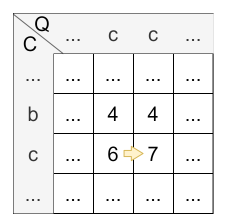
Let’s have a look at the calculation of cell \(H_{2,3}\) :
- diagonally: \(H_{1,2} + 2 * sim(b,b) = 2 + 2 * 1 = 4\)
- horizontally: \(H_{1,3} + sim(b,b) = 2 + 1 = 3\)
- vertically: \(H_{2,2} + sim(b,b) = 2 + 1 = 3\)
The maximum is 4, so the diagonal step is applied and the value of \(H_{2,3}\) is 4. The origin of \(H_{2,3}\) is \(H_{1,2}\) caused by the diagonal step.
Let’s have a look at the calculation of cell \(H_{3,3}\) :
- diagonally: \(H_{2,2} + 2 * sim(c,b) = 2 + 2 * 0 = 2\)
- horizontally: \(H_{2,3} + sim(c,b) = 4 + 0 = 4\)
- vertically: \(H_{3,2} + sim(c,b) = 2 + 0 = 2\)
The maximum is 4, so the horizontal step is applied and the value of \(H_{3,3}\) is 4. The origin of \(H_{3,3}\) is \(H_{2,3}\) caused by the horizontal step.
Let’s have a look at the calculation of cell \(H_{4,4}\) :
- diagonally: \(H_{3,3} + 2 * sim(c,c) = 4 + 2 * 1 = 6\)
- horizontally: \(H_{3,4} + sim(c,c) = 6 + 1 = 7\)
- vertically: \(H_{4,3} + sim(c,c) = 4 + 1 = 5\)
The maximum is 7, so the horizontal step, in this time a warp, is applied and the value of \(H_{4,4}\) is 7. The origin of \(H_{4,4}\) is \(H_{3,4}\) caused by the horizontal step.
Backtracking
In the last step, the cell with the highest value in the last column is the starting point of the backtracking. From there, the path is traced back to a cell where the query is indexed with 0 (the gap character). In this case, the ending point of the alignment path is \(H_{0,0}\) . The alignment path is shown in the following figure:
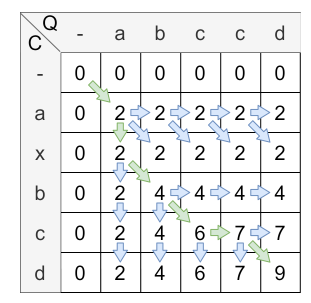
The alignment path is always unique. This path is used to calculate the similarity score. The similarity score is calculated by dividing the value of the last element from the alignment path (9) by the value of the alignment path. In this case, the value is the amount of the horizontal/vertical steps (2) added to the doubled amount of diagonal steps \(4*2=8\) . Therefore, the overall similarity score is \(\frac{9}{2+2\cdot 4} = 0.9\) .
Note that this example is based on the default values. The default values can be changed, which means that some procedures described here are no longer valid. However, this is described in more detail in the next chapter.
Implementation of the calculation #
The matrix is constructed using the following formula: \(H_{i,j} = max \begin{cases} \quad H_{i-1,j-1} + \ wTemp_i * 2 * sim_{loc}(q_i,c_j)& \text{if } x=\text{'diagonal'},\\ \quad H_{i-1,j} + \ wTemp_i * sim_{loc}(q_i,c_j)& \text{if } x=\text{'horizontal'},\\ \quad H_{i,j-1} + \ wTemp_i * sim_{loc}(q_i,c_j)& \text{if } x=\text{'vertical'},\\ \quad 0& \text{otherwise} \end{cases}\)
For further information about wTemp, read the section about the halving distance. If wTemp is not set, it is equal to 1.0.
\(q_i\) represents the i-th query item and \(c_j\) the j-th case item. \(sim_{loc}\) is the local similarity measure used.
As dynamic time warping allows warps and calculates the similarity score in the matrix differently, the alignment is included in the normalization. Let \(align =\{(0,0), \dots , (m,k)\}\) denote all cells from the alignment path. Let \(diag=\{(i_0,j_0),\dots,(i_p,j_p)\}\subseteq align\) denote all cells that originated from a diagonal step and let \(other = align \setminus diag \) denote all other assignments.
\(sim^{DTW}_{normed}(q, c) = \ \frac{sim_{raw}(q,c)}{\displaystyle\sum_{(i,j) \in diag} 2*wTemp_i + \displaystyle\sum_{(i,j) \in other} wTemp_i}\)The non normalized similarity \(sim_{raw}(q,c)\) is calculated like in the SWA.
Measure instantiation and configuration #
For this DTW-based measure, the following parameters can be set. The most parameters are described in more detail in the SWA section.
| Parameter | Type/Range | Default Value | Description |
|---|---|---|---|
| endWithQuery | Flag (boolean) | true | This parameter specifies whether the last item of the query must be in the alignment path. |
| halvingDist | Percentage (Double, [0,1]) | 0.0 | This parameter specifies the distance to the end where the events’ importance shall be one half. |
| valBelowZero | Double | 0.0 | The parameter is used to adapt the local similarity scores during calculation in the following way: \(sim_{stretched} = (1 + valBelowZero) \ast sim_{loc} - valBelowZero\) . Thereby the similarity scores will be mapped from the interval \([0,1]\) onto \([-valBelowZero,1]\) . |
| localSimName | Similarity Measure (String) | null | The parameter is used to define, which similarity has to be taken for the similarity computation between the elements of the collections. For all elements, this one local measure will be used and afterwards the global similarity is aggregated. The similarity measure, which is referred, must exist in the runtime domain, too. Otherwise, an exception will be thrown. If no localSimName is defined, a usable data class similarity will be searched. If this one can’t be found, too, an invalid similarity will be returned. |
| ignoreDifferentBeginnings | Enumeration (String) | IGNORE_DIFFERENT_BEGINNINGS_CASE | This parameter changes the similarity measure so that different beginnings are taken into account in the similarity calculation. It is possible to consider different beginnings in the case (IGNORE_DIFFERENT_BEGINNINGS_CASE), in query and case (IGNORE_DIFFERENT_BEGINNINGS_CASE_AND_QUERY) or to consider no different beginnings at all (NONE). |
| localSimilarities | Flag (boolean) | false | This parameter modifies the returned similarity object of query and case, if this parameter is set to true, the local similarities are added to the similarity object of query and case. |
The DTW-based measure can be instantiated accordingly:
    SMListDTW smListDTW = (SMListDTW) simVal.getSimilarityModel().createSimilarityMeasure(
      SMListDTW.NAME,
      ModelFactory.getDefaultModel().getClass("WeekdayList")
    );
    simVal.getSimilarityModel().addSimilarityMeasure(smListDTW, "SMListDTW");
The similarity measure can be configured using the following parameters:
endWithQuery #
By default, the final alignment must include the last item of the query, however, this behavior can be disabled:
smListDTW.setForceAlignmentEndsWithQuery(false);
halvingDist #
The halving distance can be specified as a percentage value (denoted as a value from \([0,1]\) ) of the length of the query. The distance is measured starting from the end of the query.
smListDTW.setHalvingDistancePercentage(0.5);
valBelowZero #
When using DTW, it could be essential that the scoring matrix is instantiated using negative values for punishing strong dissimilarities. Otherwise, every step in the matrix could increase the overall score. Therefore, a valBelowZero can be introduced that adapts the local similarity scores during calculation in the following way: \(sim_{stretched} = (1 + valBelowZero) \ast sim_{loc} - valBelowZero\) . Thereby the similarity scores will be mapped from the interval \([0,1]\) onto \([-valBelowZero,1]\) .
smListDTW.setValBelowZero(0.5);
localSimName #
When the local similarity to use is specified, this overwrites the configuration of the similarity model.
smListDTW.setLocalSimilarityToUse("SMStringEquals");
ignoreDifferentBeginnings #
It is possible to consider different beginnings of the similarity calculation. Possible values are: NONE, IGNORE_DIFFERENT_BEGINNINGS_CASE and IGNORE_DIFFERENT_BEGINNINGS_CASE_AND_QUERY.
smListDTW.setIgnoreDifferentBeginnings(DIFFERENT_BEGINNINGS_STRATEGIES.IGNORE_DIFFERENT_BEGINNINGS_CASE);
localSimilarities #
It is possible to calculate the local similarities of query and case, these similarities are added to the similarity object of the query and case calculation.
smListDTW.setReturnLocalSimilarities(true);
Instantiation via XML can be done as follows. Possible values for ignoreDifferentBeginnings are: none, ignore_different_beginnings_case and ignore_different_beginnings_case_and_query.
    <ListDTW name="SMListDTW"
        class="WeekdayList"
        halvingDist="0.5"
        valBelowZero="0.5"
        localSimName="SMStringEquals"
        endWithQuery="false"
        ignoreDifferentBeginnings="none"
        returnLocalSimilarities="true"/>
ListDTWWeighted #
Before reading on, please first read the basic information about the ListWeighted similarity measures.
The similarity measure ListDTWWeighted uses the similarity measure ListDTW as a basis. Here, local similarities are created, which are then used in ListDTWWeighted to offset them with the matching ListWeights.
In XML this measure can be defined as follows:
    <ListDTWWeighted name="SMListDTWWeightedXML" class="CustomListClassXML" defaultWeight="0.0" localSimName="CustomStringLevenshteinXML">
        <Weight listWeight="1.0" lowerBound="0.0" upperBound="0.1"/>
        <Weight listWeight="2.0" lowerBound="0.1" upperBound="0.6" lowerBoundInclusive="false" upperBoundInclusive="true"/>
        <Weight listWeight="4.0" lowerBound="0.6" upperBound="1.0" lowerBoundInclusive="false" upperBoundInclusive="true"/>
    </ListDTWWeighted>
At creation during runtime, the following code can be used:
    SMListDTWWeighted listDTWWeighted = (SMListDTWWeighted) simVal.getSimilarityModel().createSimilarityMeasure(
                SMListDTWWeighted.NAME, firstList.getDataClass()
    );
    listDTWWeighted.setLocalSimilarityToUse("CustomStringLevenshtein");
    simVal.getSimilarityModel().addSimilarityMeasure(listDTWWeighted, "SMListDTWWeighted");

    listDTWWeighted.addWeight(new ListWeightImpl(1.0, 0.0, 0.1));
    listDTWWeighted.addWeight(new ListWeightImpl(2.0, 0.1, 0.6, false, true));
    listDTWWeighted.addWeight(new ListWeightImpl(4.0, 0.6, 1.0, false, true));
Example: #
As local similarity measure the StringLevenshtein is used and the ListClass is utilized. Furthermore, the following intervals are given:
weight=1.0, range: [0.0, 0.1]
weight=2.0, range: (0.1, 0.6]
weight=4.0, range: (0.6, 1.0]
The DTW finds the following mapping, the local similarities are located next to the pawls:
Without the weighted approach, the similarity would be: \(\frac{4.5}{5} = 0.9\) . Considering the weights, the following similarity is calculated: \(\frac{0.5 \cdot \frac{2}{4} + 1.0 \cdot \frac{4}{4} + 1.0 \cdot \frac{4}{4} + 1.0 \cdot \frac{4}{4} +1.0 \cdot \frac{4}{4}}{\frac{2}{4} + \frac{4}{4} + \frac{4}{4} + \frac{4}{4} +\frac{4}{4}} = 0.9\overline{4}\) . As can be seen, the already high similarity with \(0.9\) can still be increased to \(0.94\) with suitable weights.
Differences SWA vs DTW #
The main difference between both approaches lies in their basic similarity assumptions. In SWA, two series are regarded as highly similar, if a sub-sequence of series A can be converted into a subseries of series B by means of as little indel operations as possible. On the other hand, DTW regards two series as highly similar, if a sub-sequence of series A can be projected onto a sub-sequence of series B by either stretching or compressing (i.e. warping) one sub-sequence onto the other. When interpreting the found alignments in the matrix for presenting them as mappings, differences emerge.
A typical mapping of SWA looks like this. Note the gap in the query that results from the deletion of Tuesday. This deletion results in a negative value being added as an indel punishment, resulting in a similarity of less than 1 in this example:
On the other hand, a typical mapping of DTW looks like this. Note that instead of deleting one Tuesday, both are warped onto the singe Tuesday of the case. This has no effect on the final similarity score, which will be 1 in this example: